Learn How to Use the FilletEdge Command

A free tutorial from Black Spectacles’ Architectural Prototyping with Rhino 5 and Grasshopper course.

In this Black Spectacles FREE tutorial, you will learn about the FilletEdge command. This tutorial is part of the Black Spectacles course on Architectural Prototyping with Rhino 5 and Grasshopper. The FilletEdge command creates a tangent surface between polysurface edges with varying radius values, then trims and joins the original faces to the fillet surfaces. View the entire course here.

The FilletEdge Command Tutorial

Step 1: Type FilletEdge in the command field to start the command

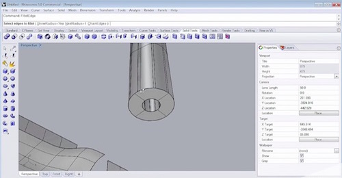
To begin, you need to have a solid object to work with. In this case we are working with a table leg. We want to give the table leg some rounded edges and to do that, we are going to use the FilletEdge command as a way of adding a radius to a series of edges in Rhino.

Step 2: Set the radius within the command

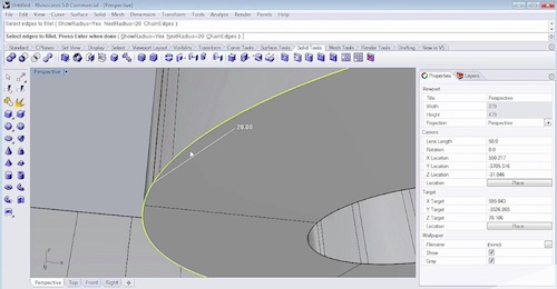
Click on ‘NextRadius=’ within the command and set it to 20 by typing 20 after ‘Next radius <1>:’ Then select the edges to fillet. Press Enter when done.

Step 3: Render the object

In the command field, select ‘SetObjectDisplayMode’. Then choose “r” (which stands for Rendered) as the mode. You will see a simulated rendered view of the object. You will end up with a nice, filleted (or rounded) edge for the table leg.

Step 4: FilletEdge the top

You can also perform this same function on the top of the table leg. However, your radius will be much smaller on the top. Repeat Step 2 for the top of your table leg, setting the radius to 5. You will end up with a nice rounded edge on the top.

Step 5: Go to shaded mode

Choose ‘SetObjectDisplayMode’ command again. But this time select “s” (for shaded) as the mode. This will set the viewpoint to an opaque, shaded mode.

Step 6: Turn off the isocurve

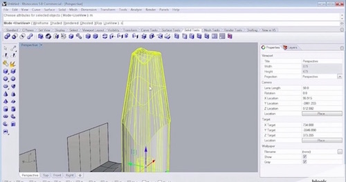
In the Properties menu on the far right, go down to the ‘Isocurve Density’ section and uncheck the box marked ‘Visible’ and this will turn off the display of your Isocurves so we can have a better view of the polysurface. 

By performing Steps 5 and 6, it allows you to see what this polysurface consists of. You can now see the seams in the object.

Step 7: Explode the object

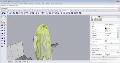
In the Command field, choose ‘Explode’. This command breaks objects down into its components and will allow you an even better image of what this closed polysurface consists of. 

You can see it’s composed of 9 individual surfaces. Below are images of 2 of them.

So you can see that as you do these transformations and modifications, your polysurfaces can become complex fairly quickly.

View the free videos in the course:

• Introduction to Complex Geometry in Rhino 5
• The FilletEdge Command
• Branch Components
• Creating Geometry for Pepakura
• Conclusion to Complex Geometry in Rhino 5